Posts

Einstein Notation
Introduction This post is written with the intention of serving as an easy reminder of how Einstein notation works for me and perhaps others who might find it useful. This is geared towards people (like myself) who want to ignore differential geometry and want to use it mainly as a simple way of expressing relatively simple computations (things like multiplying N matrices with N other matrices, perhaps summation over particular indices but not others, etc.). First, a brief description of what Einstein notation is: “a notational convention that implies summation over a set of indexed terms in a formula, thus achieving brevity” [wikipedia] Many operations like matrix multiplication, dot products, can all be thought up as “multiplying two terms from two objects and summing the result up across some axes” and Einstein notation can be used to express it in a simple and compact way. If you search up “einstein notation”, you may get results like wikipedia and youtube videos which can be confusing as they try to explain this in more general terms with respect to some concepts in differential geometry (which may not apply to your use case). Most notably, they have superscripts and subscripts to distinguish between “tangent” and “cotangent” spaces. For our purposes, we can just imagine everything is a subscript that tells us which element to look at in a multidimensional array. To add complexity to the matter, many blogposts you may find will try to explain this with respect to the numpy function einsum which is Numpy’s implementation of taking an Einstein notation formula and executing it. However, there are some differences between numpy’s implementation and how it is defined elsewhere (notably, explicit mode – as noted in the numpy documentation – has slightly different rules). For example, one main rule you will see for “classical” Einstein notation is that “an index can not repeat more than twice” – this rule is not true for numpy explicit mode. This post will focus on defining a simple set of rules for which numpy explicit mode obeys. The reason for focusing on “numpy explicit mode” rather than “classical” einstein notation is because I personally think it is easier to reason about and tools exist to parse this notation such as numpy einsum and tensorflow/pytorch einsum. Einstein Notation (numpy explicit mode) basics The rules for numpy explicit mode evaluation of einstein notation is not documented well (in my opinion) from the numpy website. This section will try to detail my understanding of it (obtained through experimentation and consolidation of other explanations found on the web). If any part of this is wrong, please reach out to me so that I can correct my understanding. At its core, einstein notation (numpy explicit mode) can describe operations of the following form: $$ A_{\color{red} \text{free indices}} = \sum_{\color{blue} \text{summation indices}} B_{\color{green}\text{b indices}} * C_{\color{violet} \text{c indices}} * … $$ We will call this equation the “Core Notation Equation” as we will be thinking of how to express operations in this form. For example, matrix multiplication is: $$ A_{\color{red}ik} = \sum_{\color{blue}j} B_{\color{green}ij} * C_{\color{violet}jk}$$ We define an output, \( A \), by noting how each element of it (\( i, k \) for matrix multiplication case) is computed with respect to entries in \( B, C, …\). We will call \( j \) a “summation” index as it is summed across and \( (i, k) \) as “free” indices to denote they are the indices that define what the output is and is “free” to vary over the output. Note: this definition of “summation” and “free” indices is very close to the wikipedia definition, but we are using it to define numpy explicit mode rules. The notation for numpy einstein notation will be: $$ {\color{green}\text{<b indices>}}\text{,} {\color{violet}\text{<c indices>}}\text{, …} \rightarrow {\color{red}\text{<free indices>}}$$ For example, matrix multiplication will be expressed as $$ {\color{green}\text{ij}}\text{,} {\color{violet}\text{jk}} \rightarrow {\color{red}\text{ik}}$$ Note that the specific letters chosen to represent an index \(i, j, k\) are arbitrary but must be consistent in the expression, so an exactly equal expression for matrix multiplication can be $$ {\color{green}\text{bc}}\text{,} {\color{violet}\text{ca}} \rightarrow {\color{red}\text{ba}}$$ Note: Numpy explicit mode happens when an arrow “->” is in the expression. If it is not, these rules do not apply. I would recommend always using numpy explicit mode. Here are some basic rules to remember this notation: Free indices are explicitly defined after the arrow (->). Summation indices are defined implicitly by all indices that are not a free. Any time a summation index appears multiple times, the notation will multiply the values together and sum across those axes. Thus, any axes addressed by the same index, say i, must have the same length. Einstein Notation Extra Information This section contains some additional information that may be helpful. Again, this applies to numpy explicit mode evaluation. If every index is free (every index to the left of “->” is also to the right of “->") then there is no summation indices to sum over. This allows an expression like “ij->ji” to express transposition. In the “Core Notation Equation” we will get something like $$ A_{ji} = B_{ij}$$ where the sum drops away because there are no summation indices. Similarily, we can extract the diagonal of a matrix into a vector with an expression like “ii->i”. The “Core Notation Equation” to think of is $$ A_{i} = B_{ii} $$ where, again, the sum drops away because there are no summation indices. If every index is summed over, then there will be no indices to the right of the “->”. This indicates we are summing over all indices. For example, an expression like “ij->” will simply sum up all the elements in the matrix. The “Core Notation Equation” here is $$ A = \sum_{ij} B_ij $$ One extra feature of numpy einstein notation is to indicate broadcasting via ellipsis. A “…” indicates all the remaining indices positionally. For example, for an N dimensional array “i…": the “…” refers to the last (N-1) dimensions “ij…": the “…” refers to the last (N-2) dimensions “…i”: the “…” refers to the first (N-1) dimensions “i…j”: the “…” refers to the middle (N-2) dimensions This is very useful when dealing with operations where the core operation is only happening in a few dimensions and every other dimension is more for “structure.” A common example is say to multiply a batch of data by a single matrix (useful for lots of neural networks) of size (N_in, N_out). The expression “…ij,jk->…ik” will work for all of the following shapes for the data: (A, N_in) : which is just singular piece of data (B, A, N_in) : a batch of B data each of shape (A, N_in) (B_1, B_2, A, N_in): a batch of (B_1*B_2) data each of shape (A, N_in) where the batch is spread over a 2d grid. Examples Matrix-Matrix Multiplication Math expression: \( A_{ik} = \sum_{j} B_{ij} * C_{jk} \) Einstein notation (numpy explicit mode): “ij,jk->ik” Matrix Hadamard Multiplication Math expression: \( A_{ij} = B_{ij} * C_{ij} \) Einstein notation (numpy explicit mode): “ij,ij->ij” Matrix-Vector Multiplication Math expression: \( A_{ik} = \sum_{j} B_{ij} * C_{j} \) Einstein notation (numpy explicit mode): “ij,j->i” Vector Dot Product Math expression: \( A = \sum_{i} B_{i} * C_{i} \) Einstein notation (numpy explicit mode): “i,i->” Sum all elements in Matrix Math expression: \( A = \sum_{ij} B_{ij} \) Einstein notation (numpy explicit mode): “ij->” Obtain the diagonal vector from a matrix Math expression: \( A_i = B_{ii} \) Einstein notation (numpy explicit mode): “ii->i” Matrix Trace Math expression: \( A = \sum_{i} B_{ii} \) Einstein notation (numpy explicit mode): “ii->” Matrix Transpose Math expression: \( A_{ji} = B_{ij} \) Einstein notation (numpy explicit mode): “ij->ji” Batch Matrix Multiplication I have a stack (size B) of matrices (each of size (N, M)) represented by a multidimensional array (B, N, M). I have a second stack (size B) of matrices (each of size (M, K)) represented by a multidimensional array (B, M, K). I want to compute an output stack (B, N, K) where the i’th matrix of shape (N, K) is computed from multiplying the i’th matrix in the first stack by the i’th matrix in the second stack. Math expression: \( A_{bnk} = \sum_{m} B_{bnm} * C_{bmk} \) Einstein notation (numpy explicit mode): “bnm,bmk->bnk” References [Youtube Video] Einstein Summation Convention: an Introduction. Faculty of Khan. [Wikipedia] Einstein Notation. [Numpy] einsum documentation. [Blog Post] EINSUM IS ALL YOU NEED - EINSTEIN SUMMATION IN DEEP LEARNING. TIM ROCKTÄSCHEL // set the pyodide files URL (packages.json, pyodide.asm.data etc) window.languagePluginUrl = 'https://cdn.jsdelivr.net/pyodide/v0.16.1/full/'; MathJax = { tex: { inlineMath: [['$', '$'], ['\\(', '\\)']], processEscapes: true, }, svg: { fontCache: 'global' }, loader: {load: ['[tex]/color', '[tex]/configMacros']}, tex: { packages: {'[+]': ['color', 'configMacros']}, }, startup:{ ready: () = { MathJax.startup.defaultReady(); MathJax.startup.promise.then(() = { resize_mathjax(); }); } } };
Circle-Circle Intersection Area
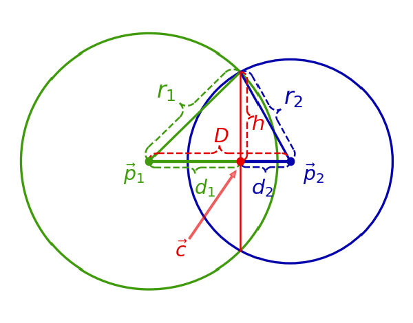
Introduction Figure 1: Area of intersection shown in orange. We look at computing the area of intersection of two circles (see Figure 1). This problem seems like it should be almost trivial. However, there are some corner cases to handle that are not immediately obvious (at least to me). Googling for this has brought me to several partial results that do not account for all the corner cases, so here is hopefully a post that is complete and can be referenced in the future to be able to quickly implement this computation. Hopefully, this post will not cause any further confusion. If you are not interested in the reading everything and just want the formulas, go to the summary. Computing the Intersection Area We consider two circles defined by their centers, \( \vec{p}_1, \vec{p}_2\) and their radiuses \(r_1, r_2\). There are some easy corner cases with the intersection of two circles: No intersection area, the circles are too far apart: \( || \vec{p}_1 - \vec{p}_2 ||_2 > r_1 + r_2\) One circle is completely inside the other (coincident circles are a special case of this), thus the intersection area is simply the area of the smaller circle \( || \vec{p}_1 - \vec{p}_2 ||_2 < |r_1 - r_2| \) One intersection point, the circles are touching at one point and have no intersection area: \( || \vec{p}_1 - \vec{p}_2 ||_2 = r_1 + r_2\) Finally, there is the “normal” case where the circle edges will intersect at two points as depicted in Figure 1. We can draw the line that contains the two intersection points, which is known as the radical axis. We can then look at computing the intersection areas on either side of the radical axis. A depiction of a possible case is shown in Figure 2. Figure 2: The total area will be the sum of the shaded areas. In this particular case, we simply need to compute the areas of the two “caps.” Each cap can be computed by subtracting a triangle from the arc area as shown in Figure 3. Figure 3: Cap area = Arc area - Triangle Area Just computing the area of the caps will not cover all cases. They represent the intersected area only when the radical axis is “in-between” the two centers of the circles. There is one more case when radical axis is not in-between the two centers of the circles. This can only happen when one circle is smaller than the other and is shown in Figure 4 (this is the case that I see most online sources miss). Figure 4: Radical axis is not in-between the circle centers. This case is still easy to deal with, as \( A_2 \) in Figure 4 is the “inverse” of the cap: the area of the smaller circle minus the area of the cap. Thus to compute the area of intersection for the case of two intersection points, we simply need to compute the area of the caps (and possibly “invert” them in the case of Figure 4). Thus, there are two cases we look at when determining the intersection area with two intersection points: The case where the radical axis is in-between the two circle centers, and the case where it is not. To compute the cap area, we need the arc area and triangle area. The arc area can be determined from the length of the chord because it will allow us to obtain the angle of the arc. The triangle area can also be determined by the length of the chord because we then have a base to an isoceles triangle. Thus we will look at computing the area of the chord. A helpful line to draw is the line connecting the two centers of the circles as shown in Figure 5. Figure 5: A helpful line and right triangles. It happens to be the case that the radical axis is perpendicular to the line connecting the circle centers [Art of Problem Solving: Radical Axis, Theorem 2]. This allows us to form right triangles as shown in Figure 5, where the hypotenuses are the radiuses of the respective circles. We can then use these right triangles to write down some geometric relationships to help us solve for the length of the chord along the radical axis. Before we write these relationships, we will now define some notation for the quantities we have been considering. Notation Figure 6: Notation. Figure 6 gives a visual guide to the various geometric quantities we will define. Note that while Figure 6 gives an example of how various geometric quantities can look, the relationships between them can change given depending on whether the radical axis is in-between the two circle centers or not. The quantities are defined as follows: Each circle is defined with a center, \( \vec{p} = (p_x, p_y)\), and a radius, \( r \). We will subscript these variables to denote either circle 1 or circle 2, e.g. \( \vec{p}_1\) is the center of circle 1. The distance between the two centers is defined as \(D = || \vec{p}_1 - \vec{p}_2||_2\) The intersection of the radical axis and the line connecting the center of the circles is denoted as \( \vec{c} \) The distance between \(\vec{c} \) and one of the intersection points is denoted as \(h\) (Note that the triangles formed by the points \(\vec{p}_1\), \(\vec{c}\), and either intersection point is the same. Thus, the quantity, \(h\), is the same no matter which intersection point you choose). The distance between \(\vec{c} \) and \(\vec{p}_1\) is denoted as \(d_1\). The distance between \(\vec{c} \) and \(\vec{p}_2\) is denoted as \(d_2\). The “Normal” Case Having defined the notation, we can start writing down geometric relationships. From the two right triangles shown in Figure 5, we can write down the Pythagorean theorem $$ \begin{align} \color{#3f9b0b} r_1^2 \color{black} &= \color{#3f9b0b} d_1^2 \color{black} + \color{red} h^2 \\ \color{#0504aa} r_2^2 \color{black} &= \color{#0504aa} d_2^2 \color{black} + \color{red} h^2 \end{align} $$ Next, one of the following equations must be true. $$ \begin{align} 1) \quad \color{#3f9b0b} d_1 \color{black} + \color{#0504aa} d_2 \color{black} &= \color{red} D \\ \color{black} 2) \color{#3f9b0b} \quad d_1 \color{black} + \color{red} D \color{black} &= \color{#0504aa} d_2\\ \color{black} 3) \color{#0504aa} \quad d_2 \color{black} + \color{red} D \color{black} &= \color{#3f9b0b} d_1 \end{align} $$ Case 1 corresponds to when the radical line is inbetween the circle centers as shown in Figure 2. Case 2 corresponds to when the radical line is not in between the circle centers (as shown in Figure 4) and circle 1 is the smaller circle Case 3 is the same as Case 2, but circle 2 is the smaller circle. Combining the two equations from Pythagorean theorem and any one of the 3 cases, we get 3 equations and 3 unknowns (\(\color{#3f9b0b} d_1\), \(\color{#0504aa} d_2\), \(\color{red} h\)). For each scenario, we can solve for \(d_1\) Click to open derivation details Looking at the two expression from the Pythagorean Theorem, we can write $$ r_1^2 - d_1^2 = r_2^2 - d_2^2$$ Looking scenario $$ d_1 + d_2 = D $$ we can write $$ \begin{align} r_1^2 - d_1^2 &= r_2^2 - (D - d_1)^2 \\ (D - d_1)^2 - d_1^2 &= r_2^2 - r_1^2\\ D^2 - 2 D d_1 &= r_2^2 - r_1^2 \\ d_1 &= \frac{r_1^2 - r_2^2 + D^2}{2 D} \end{align}$$ The other two scenarios can use a similar set of steps. $$\begin{align}1) \quad \color{#3f9b0b} d_1 \color{black} &= \frac{\color{#3f9b0b} r_1^2 \color{black} - \color{#0504aa} r_2^2 \color{black} + \color{red} D^2} {2\color{red}D} \\ 2) \quad \color{#3f9b0b} d_1 \color{black} &= \frac{\color{#0504aa} r_2^2 \color{black} - \color{#3f9b0b} r_1^2 \color{black} - \color{red} D^2} {2\color{red}D} \\ 3) \quad \color{#3f9b0b} d_1 \color{black} &= \frac{\color{#3f9b0b} r_1^2 \color{black} - \color{#0504aa} r_2^2 \color{black} - \color{red} D^2 \color{black} + 2\color{red}D} {2\color{red}D} \\ \end{align}$$ And then, solve for \(\color{red}h \) $$ \color{red}h \color{black} = \sqrt{\color{#3f9b0b}r_1^2 \color{black} - \color{#3f9b0b} d_1^2}$$ Now, we can find the area for the caps as shown in Figure 3. For circle 1, we have $$ \begin{align} Cap Area &= Arc Area \quad &- \quad&Triangle Area\\ &= \color{#3f9b0b} r_1^2\color{black} \arcsin(\frac{\color{red}h}{\color{#3f9b0b}r_1}) &- \quad&\color{red}h \color{#3f9b0b}d_1 \end{align}$$ Circle two is the same but with \(r_2\) and \(d_2\). To check if any of the caps have to be inverted, we can compute \(\color{#3f9b0b}d_1\) for the scenarios where the radial axis is not in between the circle centers. If they are not, then the value will be positive. With this, we can now compute the intersection area. Summary This section will be a succint summary of all the equations and conditions required to compute intersection area with no explanation. We use the notation introduced in Figure 6. $$\color{red}D \color{black} = || \color{#3f9b0b} \vec{p}_1 \color{black} - \color{#0504aa} \vec{p}_2 \color{black} ||_2$$ $$\color{#3f9b0b} d_{1}^{(center)} \color{black} = \frac{\color{#3f9b0b} r_1^2 \color{black} - \color{#0504aa} r_2^2 \color{black} + \color{red} D^2} {2\color{red}D}, % \quad \color{#0504aa} d_2^{(center)} \color{black} = \color{red} D\color{black} - \color{#3f9b0b} d_{1}^{(center)}, % \quad\color{red} h^{(center)} \color{black} = \sqrt{\color{#3f9b0b} r_1^2 \color{black} - \color{#3f9b0b} {d_1^{(center)}}^2\color{black}}$$ $$ \color{#3f9b0b} d_{1}^{(circle1)} \color{black} = \frac{\color{#0504aa} r_2^2 \color{black} - \color{#3f9b0b} r_1^2 \color{black} - \color{red} D^2} {2\color{red}D}, % \quad \color{#0504aa} d_2^{(circle1)} \color{black} = \color{red} D\color{black} + \color{#3f9b0b} d_{1}^{(circle1)} % \quad \color{red} h^{(circle1)} \color{black} = \sqrt{\color{#3f9b0b} r_1^2 \color{black} - \color{#3f9b0b} {d_1^{(circle1)}}^2\color{black}} $$ $$ \color{#0504aa} d_{2}^{(circle2)} \color{black} = \frac{\color{#3f9b0b} r_1^2 \color{black} - \color{#0504aa} r_2^2 \color{black} - \color{red} D^2 \color{black}} {2\color{red}D}, % \quad \color{#3f9b0b} d_1^{(circle2)} \color{black} = \color{red} D \color{black} + \color{#0504aa} d_{2}^{(circle2)} \color{black}, % \quad \color{red} h^{(circle2)} \color{black} = \sqrt{\color{#3f9b0b} r_1^2 \color{black} - \color{#3f9b0b} {d_1^{(circle2)}}^2\color{black}}$$ $$ IntersectionArea(\color{#3f9b0b}\vec{p}_1\color{black}, \color{#3f9b0b}r_1\color{black}, \color{#0504aa}\vec{p}_2\color{black}, \color{#0504aa}r_2\color{black}) = \begin{cases} % no intersection 0, & \text{if } \color{red} D \color{black} > \color{#3f9b0b} r_1 \color{black}+ \color{#0504aa} r_2\\ % one circle is smaller than the other \pi \min\{\color{#3f9b0b} r_1^2\color{black}, \color{#0504aa} r_2^2\color{black}\} & \text{if } \color{red} D \color{black} \leq |\color{#3f9b0b} r_1 \color{black} - \color{#0504aa} r_2| \\ % normal case smaller circle1 \pi \color{#3f9b0b} r_1^2 \color{black} - (\color{#3f9b0b} r_1^2 \color{black} \arcsin(\frac{\color{red}h^{(circle1)}\color{black}}{\color{#3f9b0b}r_1\color{black}}) - \color{red}h^{(circle1)} \color{#3f9b0b}d_1^{(circle1)} \color{black}) + \\ \qquad \color{#0504aa} r_2^2 \color{black} \arcsin(\frac{\color{red}h^{(circle1)}\color{black}}{\color{#0504aa}r_2\color{black}}) - \color{red}h^{(circle1)}\color{black} \color{#0504aa}d_2^{(circle1)} \color{black} & \text{if } \color{#3f9b0b} d_1^{(circle1)} \color{black} \geq 0 \\ % normal case smaller circle2 \color{#3f9b0b} r_1^2 \color{black} \arcsin(\frac{\color{red}h^{(circle2)}\color{black}}{\color{#3f9b0b}r_1\color{black}}) - \color{red}h^{(circle2)} \color{#3f9b0b}d_1^{(circle2)} \color{black} + \\ \qquad \pi \color{#0504aa} r_2^2 \color{black} - ( \color{#0504aa} r_2^2 \color{black} \arcsin(\frac{\color{red}h^{(circle2)}\color{black}}{\color{#0504aa}r_2\color{black}}) - \color{red}h^{(circle2)}\color{black} \color{#0504aa}d_2^{(circle2)} \color{black}) & \text{if } \color{#0504aa} d_2^{(circle2)} \color{black} \geq 0 \\ % normal case \color{#3f9b0b} r_1^2 \color{black} \arcsin(\frac{\color{red}h^{(center)}\color{black}}{\color{#3f9b0b}r_1\color{black}}) - \color{red}h^{(center)} \color{#3f9b0b}d_1^{(center)} \color{black} + \\ \qquad \color{#0504aa} r_2^2 \color{black} \arcsin(\frac{\color{red}h^{(center)}\color{black}}{\color{#0504aa}r_2\color{black}}) - \color{red}h^{(center)}\color{black} \color{#0504aa}d_2^{(center)} \color{black} & \text{otherwise} \\ \end{cases} $$ Concretely in python: # circle 1 radius r1 = 1.0 # circle 2 radius r2 = 0.7 def get_intersection_area(p1, r1, p2, r2): """ Computes the area of intersection between two circles. p1 and p2 are length 2 np.arrays that represent the circle center locations. r1 and r2 are their respective radiuses. """ D = np.linalg.norm(p1 - p2) if D >= (r1 + r2): # no overlap return 0 elif D < abs(r1 - r2): # one circle is fully within the other rad = np.minimum(r1, r2) return np.pi * rad**2 # intersection with two intersection points r1_sq = r1**2 r2_sq = r2**2 D_sq = D**2 invert_circle1 = False invert_circle2 = False d1 = (r2_sq - r1_sq - D_sq) / (2 * D) if d1 > 0: # The radical axis is not between the circle centers # and circle1 is the smaller circle d2 = D + d1 invert_circle1 = True else: d2 = (r1_sq - r2_sq - D_sq) / (2 * D) if d2 > 0: # The radical axis is not between the circle centers # and circle2 is the smaller circle d1 = D + d2 invert_circle2 = True else: # The radical axis is between the circle centers d1 = (r1_sq - r2_sq + D_sq) / (2*D) d2 = D - d1 h = np.sqrt(r1_sq - d1**2) area1 = (r1_sq * np.arcsin(h / r1)) - (h*d1) area2 = (r2_sq * np.arcsin(h / r2)) - (h*d2) if invert_circle2: area2 = np.pi * r2_sq - area2 elif invert_circle1: area1 = np.pi * r1_sq - area1 return area1 + area2 Submit This is an alert box. Widget Click the button to load the widget. Warning, this can lag the webpage while loading. Click This widget allows you to change and execute the python code shown in the previous section. The python code allows you to change the intersection area calculation (the output is displayed in text at the bottom of the plot) as well as the circle radiuses. You can click around the plot to change the location of the blue circle. The visualization of the red intersection area will be unaffected by the code above. To change the code, simply type in the code textbox, and press the submit button under it. Note: this widget may not work well in some mobile browsers and Safari. // set the pyodide files URL (packages.json, pyodide.asm.data etc) window.languagePluginUrl = 'https://cdn.jsdelivr.net/pyodide/v0.16.1/full/'; MathJax = { tex: { inlineMath: [['$', '$'], ['\\(', '\\)']], processEscapes: true, }, svg: { fontCache: 'global' }, loader: {load: ['[tex]/color', '[tex]/configMacros']}, tex: { packages: {'[+]': ['color', 'configMacros']}, }, startup:{ ready: () = { MathJax.startup.defaultReady(); MathJax.startup.promise.then(() = { resize_mathjax(); }); } } };
Sufficiently Accurate Model Learning
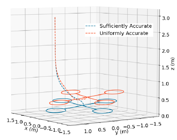
MathJax = { tex: { inlineMath: [['$', '$'], ['\\(', '\\)']], processEscapes: true, }, svg: { fontCache: 'global' }, loader: {load: ['[tex]/color', '[tex]/configMacros']}, tex: { packages: {'[+]': ['color', 'configMacros']}, }, }; Introduction This work looks at learning dynamics model for planning and control. Planners require a model of the system to work with. This model will inform the planner what happens when you take an action at some specific state. In previous work , we had applied machine learning to learn heuristics for planning. This work addresses learning the model for planning. A paper containing some results is available here. Background Planners require a model of the world that will tell us how it will evolve with certain actions. This can be expressed as a differential equation $$\dot{x} = f(x, u)$$ or as a discrete time function $$x_{k+1} = f(x_k, u_k)$$ This work will be using discrete time functions, but the ideas are more generally applicable. Many modern planners will formulate the problem as a nonlinear optimization problem, and solve it with general purpose or more specialized solvers. Examples include CHOMP, TrajOpt, or iLQG. An advantage these planners have over sampling based (such as RRT) or search based (such as A*) planners are that they perform quite admirably in high dimensions and converge quickly to locally optimal solutions. These optimization planners only work in “relatively” simple environments. Problems where finding the solution might require a search through many homotopy classes are difficult for this class of optimization based planners. They require a decent initialization. But, as it turns out, for many real world situations, planning is more akin to optimizing a general idea of what to do, rather than solving a complicated maze. One can try to use data to obtain a better model for planning with these optimization based planners. Usually the constraints on the model are that they have to be differentiable. Using a neural network to represent these models fits this constraint quite well. By using data to tune or learn your model, you can have a more accurate picture of what your system looks like and adapt to any physical changes it undergoes. Maybe the wheel of a car becomes more smooth over time, or a motor in a robot arm becomes less powerful. By using data, the planners can adapt to these changes in a more active way. There is a vast literature on model learning. In controls, there is a huge trove of “System Identification” papers which mostly focus on learning linear systems. In robotics, there are many methods that fit Gaussian Process Regression models, or Gaussian Mixture Models, or Neural Networks, or linear models to various systems. This paper presents not a new method, but a new objective for which these methods can use. Most of these methods will simply seek to minimize an error between an observed next state, \(x_{k+1}\) with that the predicted next state, \(\hat{x}_{k+1}\). This results in a loss functions that look like $$ \mathbb{E} || x_{k+1} - f_\theta(x_k, u_k) ||_2^2$$ where \(f_\theta\) is the learned model. Method Our work proposes that we can solve a constrained problem instead of simply minimizing an unconstrained objective. The constraints can contain prior information about the system, and solving the constrained problem can then lead to models better suited for planners. An simple example is suppose we have a block we are pushing on a table, that has lot of uneven surfaces. Suppose we want to push the block from various points to a common resting location. We can learn a model that is uniformly accurate everywhere. Or, we can learn a model that is selectively good near the goal location. Because far away from the goal, the plan is simple, we push in the direction of the goal. It is only when we are near the goal we care about how much we push so that the block comes to a stop efficiently and correctly. This prior knowledge can be summarized as a constraint on the accuracy near the goal. We can write a constrained problem that looks like $$ min_\theta \mathbb{E} f(x_k, u_k, x_{k+1})\ s.t. \mathbb{E} g(x_k, u_k, x_{k+1}) \leq 0$$ We have explored solving constrained problems before . In this case, we expand the theory somewhat. We can no longer analytically compute the expectations in the constrained problem and can only use samples of data. This is because the distribution of trajectories for a system is very complicated. This paper shows that you can still obtain small duality gaps with large enough models and large enough numbers of samples. Similar to our previous work , we can use a primal-dual method to solve this. We alternatively minimize the Lagrangian, and maximize the dual variables. Results Using some constrained objectives, we can obtain models so that the planner can do better on average. We have tested this in simulation on a state-dependent-friction block pushing task, a ball bouncing task, and a quadrotor landing task. Numerical results show that we can trade off accuracy in unimportant parts of the statespace for better accuracy in others, and obtain better performing planners. The detailed results are under submission right now. But to highlight a few instances for why this is better, we can look at the quadrotor landing. Our constraint is that the model should be more accurate close to the ground. This is where ground effects are most prominant and require greater precision in the model. Fig. 1: Quadrotor trajectories. A model learned using our objective is better able to compensate for the greater updraft near the ground when landing and can get to the location more accurately. References Zhang, Clark, and Paternain, Santiago, & Ribeiro, Alejandro. Sufficiently Accurate Model Learning for Planning. 2021. Zucker, Matt, et al. “Chomp: Covariant hamiltonian optimization for motion planning.” The International Journal of Robotics Research 32.9-10 (2013): 1164-1193. Schulman, John, et al. “Finding Locally Optimal, Collision-Free Trajectories with Sequential Convex Optimization.” Robotics: science and systems. Vol. 9. No. 1. 2013.< /a> Todorov, Emanuel, and Weiwei Li. “A generalized iterative LQG method for locally-optimal feedback control of constrained nonlinear stochastic systems.” Proceedings of the 2005, American Control Conference, 2005.. IEEE, 2005.
Learning Implicit Sampling Distributions
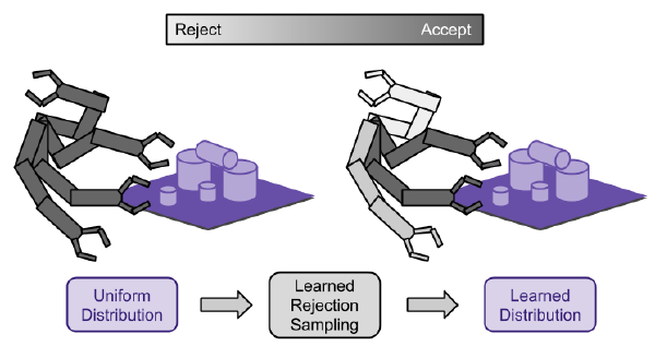
MathJax = { tex: { inlineMath: [['$', '$'], ['\\(', '\\)']], processEscapes: true, }, svg: { fontCache: 'global' }, loader: {load: ['[tex]/color', '[tex]/configMacros']}, tex: { packages: {'[+]': ['color', 'configMacros']}, }, }; Introduction Robot motion planning is a problem that has been studied for many decades. For quite a while, sampling based planning approaches such as Rapidly Exploring Random Trees (RRT), Expansive Space Trees (EST), were quite popular in academia have been used with great success in some problem domains. This post introduces work I have done in collaboration with Jinwook Huh and Daniel D. Lee about speeding up such motion planning approaches by learning a better sampling distribution to draw from. This work is available here. While many more modern planners for robots such as autonomous vehicles no longer have a basis in these sampling based planners, perhaps similar ideas in how to integrate machine learning into an existing planning framework can be useful. Background We can discuss a bare-bones planning problem. You have a map of the environment that can be represented maybe as a point cloud or occupancy map or collection of polygons, or a signed distance function, etc. You have a goal state and a starting state, and you would like to find a set of actions for a robot that will take you from start to goal. Fig. 1: An example of a planning problem. The green dot is the start, while the red is the goal. For sampling-based planners, the general idea is to explore a continuous state space with random samples. The prototypical sampling based planner, RRT, roughly works as follows. Initialize a tree with a node that represents the starting state Sample a point in the entire state space Find the closest node in your tree to the sample From the closest point, move towards the random sample and add the new state as a node in the tree Repeat steps 2-4 until the goal is included in the tree. This process will grow the tree to cover the space and hopefully find a path from the start to the goal. You can check out Steven LaValle’s website (The guy who invented RRT’s) for cool pictures of RRT in action and what it looks like while the algorithm is running. For these sampling based planners, Step 2 in the algorithm can be quite important. It is what will guide how the tree searches the environment (if you are familiar with A* and its many variants, the sampling distribution plays a similar role to the heuristic function). Typically, a uniform distribution with a slight goal bias (with some chance, choose the goal as the random sample) is used. There have been many efforts to come up with better sampling techniques including using the medial axis, visibility, or volumes. These are all heuristics that hopefully are better distributions to sample from than the uniform distribution. A natural question arises, can we learn more general heuristics for common classes of planning problems? For example, if we are using a robot arm to manipulate objects on a table, we might be able to exploit some of the structure of the problem to speed up our search. This heuristic may be different if you are talking about a robot navigating an office space, or an autonomous vehicle navigating around a city. And it would be great to use data from planning in those different environments to learn good sample distribution. Method To learn a sampling distribution, we must first be able to represent a sampling distribution. In this case, we have chosen to represent it implicitly (thus the title of the paper) with rejection sampling. That is, given some simple distribution that you can easily draw samples from (uniform with goal bias), assign a probability of rejecting that sample. Then when you are sampling from this implicitly defined distribution, you will draw samples from the original distribution and with some probability, reject on those samples. This will define a new distribution that can look quite different from the original distribution with out rejecting any samples. In this particular case, we use a small (tiny by modern standards) neural network to process some features of a sample drawn. The output of the neural network is a probability to accept or reject. Fig. 2: A tiny neural network. We can then view the process of accepting and rejecting samples to pass to the planner as a Markov Decision Process (MDP) where the state is the state of the planner with a new random sample, and the actions are to reject or accept it. The rewards are chosen to reward finding a path faster. This process can be optimized with some standard Reinforcement Learning (RL) techniques. There are a great many tutorials and introductions to RL, so I will abstain from adding one more slightly worse introduction. I highly recommend this book by Sutton as a good introductory read. For our purpoes, we will use a simple policy gradient method to optimize our rejection “policy.” Results This methodology is applied to several environments and algorithms and the results are shown in Fig. 3. In addition to RRT, you can apply this rejection sampling technique to any other sampling-based planner such as Bi-RRT or EST, etc. The flytrap environment refers to Fig. 1, while Pendulum referes to an inverted pendulum. Fig. 3: Results in simulation. We also applied this to a robot arm in real life. Fig. 4: Thor's robot arm. Fig. 5: Results on a robot arm. In these cases, the new sampling distribution can reduce the number of collision checks by rejecting samples that are highly likely to induce them as well as reducing overall execution time. It is also interesting to look at the learned rejection policies more closely. For the flytrap environment, good rejection policies actually depend on the size of the flytrap relative to the environment. The visibility based heuristic works when the flytrap is small, and the volume based heuristic works when the flytrap is big. When running the rejection policy optimization over small and big flytrap environments, it actually obtains very similar heuristics to the human created ones. Fig. 6: Learned rejection policies vs. human heuristics. Flytrap train refers to the small flytrap, dynamic-domain refers to the visibility heuristic, flytrap-balltree refers to the big flytrap, and BallTree refers to the volume based heuristic. Fig. 7: Cool sampling distributions in action on the flytrap environment. For the robotic arm, when we look at the learned distribution, the samples that are further away from the table are rejected more often. For the task of moving objects around, it is wasteful to explore random configurations that bring the arm way over or away from the objects. Conclusion This work had the goal to unify the understanding of how a lot of previous sampling heuristics worked. Many use rejection sampling, and Reinforcement Learning can be applied to optimize that rejection sampling so as to automate the process of finding heuristics. There are some interesting tangents to discuss. For example, if an optimal planner is available (RRT* and friends), instead of using RL to optimize rejection policies, supervised learning can be used instead. With supervision, the policies can be learned faster, and perhaps, we can obtain even better policies. For complicated environments, however, RRT* can take very long to run. It can be interesting to start with RL and move to supervised learning as our heuristics get better and we can find near-optimal policies. Since this paper’s publication, there has been interesting work in learning heurstics for A*, as well as generative sampling distributions. References Zhang, Clark, Jinwook Huh, and Daniel D. Lee. “Learning implicit sampling distributions for motion planning.” 2018 IEEE/RSJ International Conference on Intelligent Robots and Systems (IROS). IEEE, 2018. Y. Yang and O. Brock, “Adapting the sampling distribution in prm planners based on an approximated medial axis,” in Robotics and Automation, 2004. Proceedings. ICRA’04. 2004 IEEE International Conference on, vol. 5, pp. 4405–4410, IEEE, 2004. A. Yershova, L. Jaillet, T. Siméon, and S. M. LaValle, “Dynamic- domain rrts: Efficient exploration by controlling the sampling domain,” in Robotics and Automation, 2005. ICRA 2005. Proceedings of the 2005 IEEE International Conference on, pp. 3856–3861, IEEE, 2005. A. Shkolnik and R. Tedrake, “Sample-based planning with volumes in configuration space,” arXiv preprint arXiv:1109.3145, 2011. Sutton, R. S., Barto, A. G. (2018 ). Reinforcement Learning: An Introduction. The MIT Press. Zlatan Ajanovic, Halil Beglerovic, Bakir Lacevic. “A novel approach to model exploration for value function learning.” RSS 2019 workshop. Ichter, Brian, James Harrison, and Marco Pavone. “Learning sampling distributions for robot motion planning.” 2018 IEEE International Conference on Robotics and Automation (ICRA). IEEE, 2018.
Constrained Learning for Wireless Systems
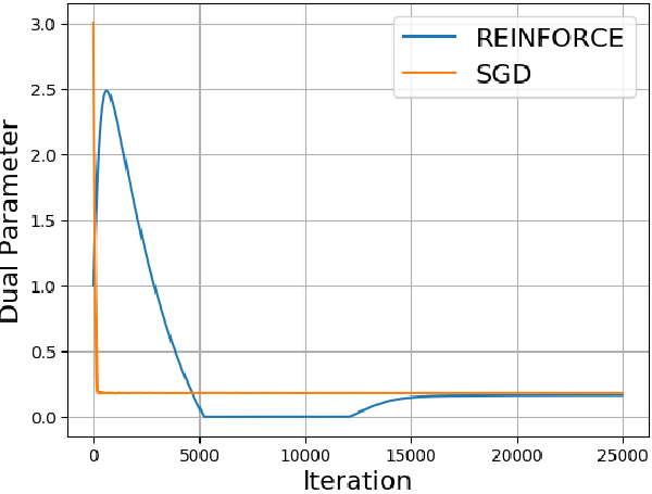
MathJax = { tex: { inlineMath: [['$', '$'], ['\\(', '\\)']], processEscapes: true, }, svg: { fontCache: 'global' }, loader: {load: ['[tex]/color', '[tex]/configMacros']}, tex: { packages: {'[+]': ['color', 'configMacros']}, }, }; Introduction This post introduces some work done in collaboration with Mark Eisen about solving optimization problems of the form $$min_\theta \text{ } E_h[l(h, f_\theta(h))] \ s.t. E_h[g(h, f_\theta(h))] \leq 0$$ where \( l \) is a smooth loss function, and \(g\) is a smooth constraint function. In particular, this optimization has to be done where \(l\) and \(g\) may be unknown or hard to measure. This is the case for wireless power allocation. One goal is to maximize throughput while under power constraints. The throughput is affected by the environment (how the waves bounce around, other wireless interference, etc.) which can be changing over time. The characterstics of the environment can be measured, but not so easily, and it can change quite fast. Thus, Reinforcement Learning (RL) seems to be a good candidate solution. However, most Reinforcement learning algorithms do not optimize with constraints in mind. This work will extend common methods into constrained versions. Our paper is available here. Background I am not an expert in wireless technology. So for a more complete picture, I will point you to examples in our paper that my coauthor has written. A brief summary will be that wireless transceivers have a variety of channels (frequency allocations) on which it can choose to communicate on. The channels are effected by \(h\), the fading. Generally, sending a more powerful signal will allow the message to be recieved with greater probability, though other transmitters might interfere as well. The goal is to allocate power to multiple transmitters across channels to maximize throughput while obeying a power constraint. Reinforcement learning is a technique to solve Markov Decision Processes (MDP) when some part of the MDP is unknown. There are many great resources for an intro into reinforcement learning such as this book. I will abstain from adding one more slightly worse introduction. Method We use policy gradient methods from Reinforcement Learning to find a good policy for wireless allocation. The policy is stochastic, and takes a measurement of the fading environment as input. The output is a distribution over power allocations, represented by the parameters of a truncated Gaussian. Because we have a constrained problem, just applying policy gradient doesn’t work. Instead, we look at the dual problem. If you are unfamiliar with optimization and duality, this is a large topic to try to breach here. A high level overview is that optimization problems can be represented in a different (dual) form that may be easier to solve. This dual form takes the constraints of the original and puts it into the objective. The optimization is then done over Lagrange multipliers. One thing to note is that solving the dual problem is not always the same as solving the original problem. In the case of convex problems, they are the same. This paper shows that with large enough neural networks to represent the policy, the dual problem is almost the same as solving the original. The dual problem looks like this $$max_\lambda min_\theta E_h[l(h, f_\theta(h))] + \lambda^T E_h[g(h, f_\theta(h))]\ s.t. \lambda \geq 0 $$ There is a maximization over the Lagrange multipliers, \(\lambda\), and a minimization over the parameters of the policy, \(\theta\). We can treat the Lagrangian (everything within the max-min) as a reward for policy optimizaiton. We can then interleave minimizations, by taking steps with the policy gradient, with maximizations with respect to the lagrange multipliers. This way of alternating optimizations is known as a primal-dual method, and is known method in optimization. Results Fig. 1 shows the results of our experiments. We simulated wireless channels with noise, and compared some strategies with the learned policy. The x axis represents time. Our policy gets better with time as it learns from the accumulated experience. The strategies compared with are 1) random allocation, 2) equal power allocation, 3) WMMSE. WWMSE is a state-of-the-art method that requires a model of the capacity function (which our method does not have access to). We can do this in simulation, because we can choose a capacity function and give it to WWMSE. The graphs show that we can obtain comparable performance to WMMSE without having to model the capacity function. Fig. 1: Results of applying our method on a wireless channel simulation. Conclusion This work shows that there is some promise in using Reinforcement Learning to optimize wireless power allocation. Since this paper’s publication, Mark has extended it to use graph neural networks. References Eisen, Mark, et al. “Learning optimal resource allocations in wireless systems.” IEEE Transactions on Signal Processing 67.10 (2019): 2775-2790. Sutton, R. S., Barto, A. G. (2018 ). Reinforcement Learning: An Introduction. The MIT Press. Eisen, Mark, and Alejandro R. Ribeiro. “Optimal wireless resource allocation with random edge graph neural networks.” IEEE Transactions on Signal Processing (2020).

Pyodide test
Testing pyodide, the cpython interpreter compiled to webasm. Quick test of a 3 link robot arm. // set the pyodide files URL (packages.json, pyodide.asm.data etc) window.languagePluginUrl = 'https://cdn.jsdelivr.net/pyodide/v0.16.1/full/'; Type Python code here # you can modify the arm lengths here and then press submit arm.lengths = np.array([1., 1., 1.]) Loading -- theta0 theta1 theta2 var editor = ace.edit("editor"); editor.getSession().setMode("ace/mode/python"); editor.setTheme("ace/theme/monokai"); setup_script = `import numpy as np import matplotlib.pyplot as plt from js import document import io import base64 class Arm(object): def __init__(self): self.lengths = np.array([1., 1., 1.]) self.lines = None self.pts = None def fwd_kinematics(self, thetas): cum_thetas = np.cumsum(thetas) x_diffs = self.lengths * np.cos(cum_thetas) y_diffs = self.lengths * np.sin(cum_thetas) x_coords = np.cumsum(x_diffs) y_coords = np.cumsum(y_diffs) coords = np.stack((x_coords, y_coords), axis=1) coords = np.concatenate((np.array([[0., 0.]]), coords), axis=0) return coords def draw(self, ax, thetas): coords = self.fwd_kinematics(thetas) assert(len(coords) == 4) if self.lines is None: self.lines = [] for i in range(3): self.lines.append(ax.plot([0, 1], [0, 1], c="b")[0]) self.pts = ax.scatter([0, 0, 0, 0], [0, 0, 0, 0], c="g") for i in range(len(coords) - 1): pt1 = coords[i, :] pt2 = coords[i+1, :] self.lines[i].set_data([pt1[0], pt2[0]], [pt1[1], pt2[1]]) self.pts.set_offsets(coords) ax.set_xlim([-4, 4]) ax.set_ylim([-4, 4]) ax.set_aspect('equal', 'box') #ordinary function to find an existing div #you'll need to put a div with appropriate id somewhere in the document def create_root_element2(self): return document.getElementById('arm-figure1') arm = Arm() f = plt.figure() print(dir(f.canvas)) #override create_root_element method of canvas by one of the functions above f.canvas.create_root_element = create_root_element2.__get__( create_root_element2, f.canvas.__class__) ax = f.gca() ax.grid() theta0 = float(document.getElementById("arm-theta0").value) theta1 = float(document.getElementById("arm-theta1").value) theta2 = float(document.getElementById("arm-theta2").value) thetas = [theta0, theta1, theta2] arm.draw(ax, thetas) f.canvas.show() #buf = io.BytesIO() #plt.savefig(buf, format='png') #buf.seek(0) #img_str = "data:image/png;base64," + base64.b64encode(buf.read()).decode('UTF-8') #img_tag = document.getElementById("arm-figure1") #img_tag.src = img_str #buf.close()` theta_change_script = ` theta0 = float(document.getElementById("arm-theta0").value) theta1 = float(document.getElementById("arm-theta1").value) theta2 = float(document.getElementById("arm-theta2").value) thetas = [theta0, theta1, theta2] arm.draw(ax, thetas) f.canvas.show() ` function setup_slider_cbs() { $("#arm-theta0").on("change", ()={ pyodide.runPythonAsync(theta_change_script) .then(()={}) .catch(()={}); }); $("#arm-theta1").on("change", ()={ pyodide.runPythonAsync(theta_change_script) .then(()={}) .catch(()={}); }); $("#arm-theta2").on("change", ()={ pyodide.runPythonAsync(theta_change_script) .then(()={}) .catch(()={}); }); }; languagePluginLoader.then(() = { pyodide.runPythonAsync(setup_script) .then( (output)={ console.log(output); $("#output").val("Ready\n"); setup_slider_cbs();} ) .catch( (err)={console.log(err);}); }); $("#button").click(function() { pyodide.runPythonAsync(editor.getValue() + "\n" + theta_change_script) .then(function(output) {$("#output").val($("#output").val() + "\n" + String(output));}) .catch(function(err) {$("#output").val($("#output").val() + "\n" + String(err));}); });